Carrier Single Differencing

This segment of the LEOGPS documentation gets into the technicals of baseline estimation between formation flying satellites (or even between static stations in general), and it assumes that the user has sufficient knowledge on single-point positioning concepts. The algorithm described in this section is based on carrier phase differencing, and is largely implemented in the code file ambest.py (ambiguity estimation). For a tutorial on the more basic aspects of GNSS, the user is invited to peruse ESA’s NaviPedia.

Carrier phase differential GPS, or CDGPS in summary, is the technique of estimating the relative position of a receiver with respect to another, over a short baseline. The carrier signal’s phase is typically exploited for precise point positioning due to its ranging precision, rather than using the unambiguous code. In the case of GPS signals, the ranging accuracy of the C/A code signal is typically on the order of ±3m for a typical GNSS receiver (on the modernized GPS block without selective availability); whereas the ranging accuracy of the carrier phase of the signal is on the order of millimeters due to the relatively short wavelength (19.05cm for L1 for example) and the accuracy achievable in most receiver phase-locked loops today.

The carrier phase range can be modelled as the observed phase, plus an integer number of wavelengths, and plus a series of systematic and random ranging errors. The goal of carrier phase differential GPS techniques is to remove these systematic ranging errors through differential measurements which cancel common and correlated sources of ranging errors observed by both receivers over a “short” baseline.

The integer number of wavelengths however, is unknown and must be estimated. This is known as the “integer ambiguity resolution” problem in GNSS literature, and it can be estimated as a float, with subsequent integer fixing techniques (i.e., wide-lane, narrow-lane, or if the error covariances are known, then integer fixing by Peter Teunissen’s LAMBDA).

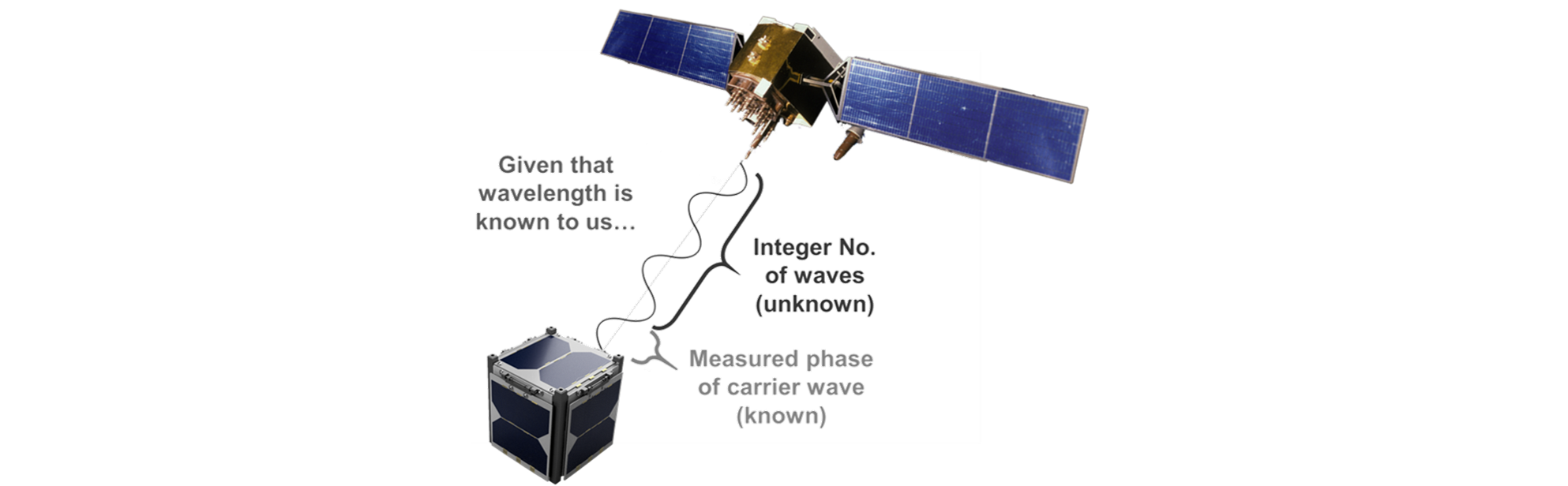
_images/leogps_0diff_fig1.png — Figure C1.1: Carrier phase ranging illustration highlighting the ambiguity N.

In any case, the receiver end only measures the instantaneous carrier phase modulo 360 degrees. It is unknown to the receiver how many integer cycles of the carrier signal has passed through the signal path taken from the emission from the GPS satellite to the receiver. Nevertheless, the RINEX file carrier phase observable would normally give an integer estimate nonetheless (usually using a pseudo-range model).

In order to very accurately characterize the range, the number of integer cycles, hereby known as N, must be made known. The integer ambiguity of the carrier phase is red-boxed below.

_images/leogps_0diff_eqn1.png — Equation C1.1: Carrier phase ranging model

On top of the integer ambiguity N, there are various other error sources that are modelled in the GPS signal range equation (Equation C1.1), of which are the following in descending order of importance and accuracy loss: the GPS satellite clock bias estimation errors, the LEO satellite clock bias, ionospheric path delays, and other relativistic effects such as clock advance effects and Shapiro path delays.

The key to mitigating errors is the realization that error components shown in Equation C1.1, are highly correlated among GPS receivers in proximity. Subtracting measurements (differencing) between receivers will therefore “cancel” out systematic errors between the LEO satellites.

_images/leogps_1diff_fig1.png — Figure C1.2: Carrier phase single differencing between two LEOs

In the case of the single differencing scenarios, the absolute carrier phase measurements taken by two LEOs are subtracted from each other. Using the carrier phase ranging model from Equation C1.1, the error sources that are common to both are red-boxed below.

_images/leogps_1diff_eqn1.png — Equation C1.2: Common errors for a single differencing scenario

Since the baseline of the LEO satellites are expected not to deviate beyond 200km, it is considered “short”, and thus likely that the ionospheric errors are correlated. Also, this means that the total number of and pseudo-range IDs of GPS satellites in view will not be any different between the two LEOs. Thus, in the single differencing case, between two LEOs and some k-th GPS satellite, differencing the carrier phase measurements between LEO A and B will remove systematic biases in ionospheric path delays, the k-th GPS satellite clock offsets, and common relativistic effects.

_images/leogps_1diff_eqn2.png — Equation C1.3: Carrier phase single differencing equation

As a result, the single difference equation comprises only of the relative true ranges, the relative receiver clock bias estimation errors, and the relative carrier phase cycle integer ambiguities. For the epsilon error term, assuming both errors are Gaussian, this results also in a square-root-2 amplification in white Gaussian noise.

If the receiver clock bias errors are small, then the baseline can actually already be derived from the single difference equation with little consequence to the accuracy of the baseline AB.

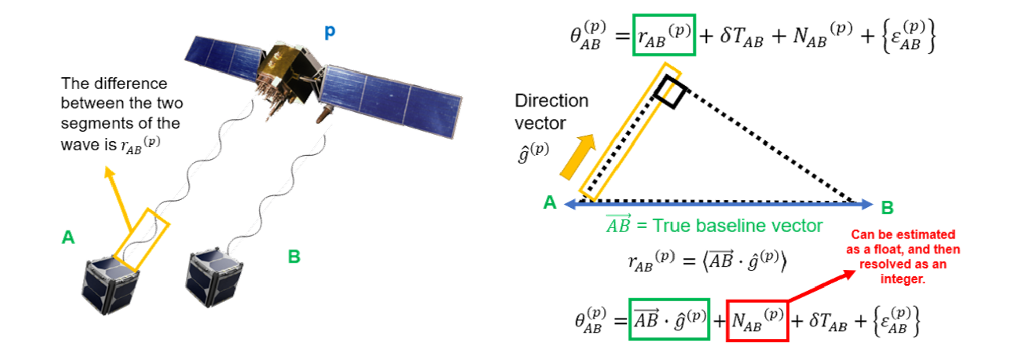
_images/leogps_1diff_fig2.png — Figure C1.3: Extraction of baseline vector AB from the single differencing equation.

In extracting the baseline vector AB in Figure C1.3, the experimenter makes a few assumptions. First, assume that the GPS satellite is far away enough such that the signal paths taken from the emitter to the receivers A and B are almost parallel. Second, assume also that the receiver will be able to estimate the direction vector from itself to the GPS satellite, which is given by g-hat in the Figure C1.3, without introducing new errors. This is possible only if coarse positioning estimates of itself is first achieved using the C/A or P code, and that the GPS navigation observables are correctly parsed. In most cases, since the distance of the GPS satellite to the LEO is on the order of about ~20,000km, any coarse positioning errors on the meter-level scale would not significantly affect the accuracy of the estimation of the g-hat vector. Next, a very rough estimate of the integer ambiguity can be estimated as a float using the pseudo-range values ρ from code measurements, and the known carrier wavelength λ.

One can now solve for the AB vector as seen in Figure C1.3, notwithstanding the fact that the receiver clock bias estimation errors were not cancelled out and will thus show up in some form in the accuracy of the positions. The single differenced baseline solution from LEOGPS for a 100km baseline separation is shown below:

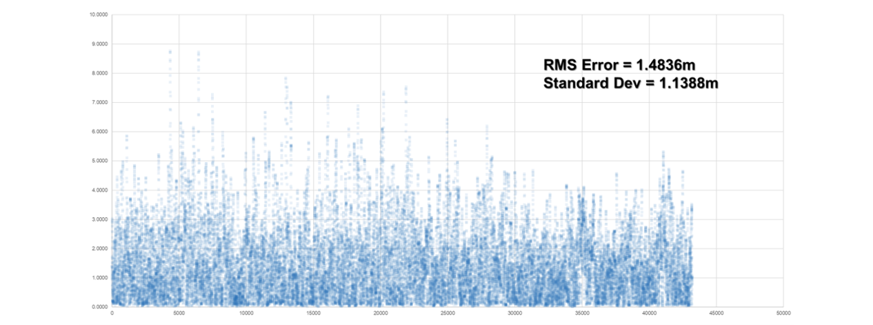
_images/leogps_1diff_plot.png — Figure C1.4: Relative position error norm of a single differenced 100km LEO baseline.

Observably, the single differenced solution still faces an accuracy > 1m. Embedded in the error plots are likely the unaccounted relative receiver clock bias estimation errors, minor error sources such as antenna phase centre variations, et cetera, which were not differenced away, as well as other white noise error sources.

Note

Every step of differencing amplifies the random error sources by root-2, assuming the noises are well-modelled as a Gaussian.

We can go a step further to difference a pair of single-difference observations in order to eliminate the remnant relative receiver clock bias estimation errors. This technique is known as double-differencing, and it will be explained in the next section.